Teleseismic Depth Phases
In most location codes teleseismic depth phases are handled like any other phase; a residual is computed against a standard traveltime model and then the hypocenter (especially focal depth) is adjusted to reduce the misfit. If the theoretical traveltime of the teleseimic P portion of the pP raypath exhibits any bias with respect to the true traveltime, however, the inferred focal depth will also be biased. In fact the teleseismic P branch in calibrated clusters is typically found to be biased (relative to ak135) by several seconds, as seen in this example from the Ridgecrest, California cluster. If the focal depth were based on fitting the observed pP and sP arrivals, it would be over-estimated.
For this reason, mloc converts the main teleseismic depth phase readings into relative depth phases pP-P and sP-P for analysis, removing most bias from the teleseismic P branch. The water-multiple pwP phase is also processed as the differential phase pwP-P. Any other depth phases encountered (e.g., sS, pPn, pPKP, etc) will be processed “normally” if they exist in the phase set or flagged (with “p”) if not. A section of the ~.log file lists the converted relative depth phases. The main source of information is the ~.depth_phases file.
The analysis described here has to be conducted outside the actual relocation, and the results brought into subsequent relocation runs by setting the depth with the depd command and relocating with fixed depth. Depth constraints from teleseismic depth phases cannot usually be utilized in a free-depth relocation (other than as starting depths) because the data are few in number and sparsely-distributed among events.
Bogus Depth Phase Readings
It has recently become known that certain seismograph stations have been reporting fictitious depth phase readings to the ISC and perhaps other data centers. It appears that analysts at these stations (or perhaps a regional data center) have been reporting theoretical arrival times of depth phases based on a preliminary hypocenter. A characteristic sign of this issue is to find several stations reporting both pP and sP with times that match perfectly with each other. It appears this problem began somewhere around the year 2000 but it may well be station-specific.
In mloc this problem is dealt with by maintaining a file of stations suspected of reporting bogus depth phase readings, which is referenced by the command bdps. It is strongly recommended to use this command for any cluster in which depth phase analysis will be employed to constrain depths. Data from suspected stations will be flagged in the depth phase analysis to prevent its use.
As a review of the file bdps.dat will show, the stations so far suspected of reporting bogus depth phase data are all in China, but there have been fears about this ever since routine analysis has come to be done with computer software capable of over-laying theoretical arrival times on observed records. There may well be other sources of spurious readings so vigilance is recommended.
Best-Fitting Depth
The method used in mloc to determine the optimal focal depth from reported depth phases is based on an important principle: that the reported phase names for depth phases from standard seismic bulletins cannot be trusted. That the reported arrival is even a proper depth phase is in considerable doubt but the phase names reported are so often in error that they should generally be ignored. This principle was established by E.R. Engdahl during his work on the EHB catalog, in which careful inspection of reported depth phases is a key element of the improved focal depth estimates for which that catalog is known.
After each run of mloc a trial is conducted over a range of depths (1-99 km, limits hard-coded in mloc.f90) to find the best fit to observed relative depth phases. At each trial depth, and for each relative depth phase time difference, the theoretical traveltime difference is calculated for all supported relative depth phase identifications: pP-P, sP-P and pwP-P. The phase with minimum residual is selected, whether or not the phase name is consistent with the original report. The total RMS error from all depth phases is calculated at each trial depth, and the depth with minimum cumulative error is taken as optimal for that event in that run of mloc. The asymmetric uncertainty in depth (at ~90% confidence level) is calculated using the zM test (e.g., Langley, ‘Practical Statistics, Simply Explained’, Dover Publications, 1970, p 152.), to find the range of depths around the preferred depth in which the z statistic, relative to the value of z at the preferred depth, is less than the value at which the null hypothesis (no difference) would be rejected at the 10% level of probability.
The z Test for Measurement (hence ‘zM’) compares a random sample of one or more measurements with a large parent group whose mean and standard deviation are known.
The statistic z is calculated from z = (sqrt(n)·abs(M-m))/S, where:
- n = number of measurements in the sample
- m = mean of the sample measurements
- M = mean of the parent group
- S = standard deviation of the parent group
The probability of no significant difference between M and m at the 10% level of confidence is 1.64. This value is added to the value of z calculated for the depth at which z is a minimum to estimate the uncertainty range for focal depth. We assume M = 0.0. because we expect the relative depth phase residuals to have zero mean at the true depth. The specification of S is more problematic. The code assume S = 1., which seems sensible based on looking at residuals of many depth phase readings, but further investigation is warranted. This analysis is still relatively new in mloc and when a larger set of results is available this parameter may be revised.
The output from the test described above often reveals outlier readings which account for an inordinate proportion of the cumulative error. A cleaning process, i.e. flagging the outliers and re-running mloc, is used to bring the depth phase data into a self-consistent state. The process is somewhat subjective and experience with many events will lead to a good instinct for what can expected from standard (e.g., ISC-sourced) datasets.
It is certainly true that this analysis for focal depth can be criticized from several points of view but the results are generally consistent with other estimates of focal depth (when they exist) and with our expectations of what can reasonably be expected in terms of precision from the depth phase data extracted from standard global catalogs. Traditionally, this kind of fitting has been done “by eyeball”. These are initial steps to try to put the analysis on a more statistically-driven footing.
Depth Phase Analysis Output
The results of the analysis described above are presented in two ways. Details for each event are listed in the beginning of the ~.depth_phases output file and the error-vs-depth curve is optionally plotted using the rdpp command. Here is an example of the file output, for the Ridgecrest, California cluster:
  4 19950920.2327.35               preferred depth =  24 km ( 13 to  30) on   1 samples (depd  24  6 11)
 11 19961127.2017.24               preferred depth =   8 km (  4 to  17) on   1 samples (depd   8  9  4)
 27 20190704.1733.49               preferred depth =  19 km ( 12 to  23) on   4 samples (depd  19  4  7)
 45 20190706.0319.52               preferred depth =  22 km ( 13 to  26) on   5 samples (depd  22  4  9)

Residuals against each theoretical phase for the depth with minimum misfit
                        MNF      pP-P      sP-P     pwP-P     Err**2
Event   4 19950920.2327.35                 24 km
  GRF   83.65 sP-P      261      0.04     -2.90      0.04      0.00   pP-P
Event  11 19961127.2017.24                  8 km
  LVZ   74.26 sP-P      170      1.12     -0.02      1.12      0.00
Event  27 20190704.1733.49                 19 km
  ARCES 71.62 pP-P      644     -4.06     -6.26     -4.06     16.47 x
  EKA   73.43 pP-P      648     -0.11     -2.48     -0.11      0.01
  EKA   73.43 pP-P      649      0.04     -2.33      0.04      0.00
  EKA   73.43 sP-P      650      3.06      0.69      3.06      0.48
  NB2   74.94 sP-P      664      5.22      3.04      5.22      9.21 x
  HFA0  76.42 pP-P      679     -2.86     -5.04     -2.86      8.16 x
  FINES 78.76 pP-P      682     -0.76     -2.94     -0.76      0.58
Event  45 20190706.0319.52                 22 km
  ARCES 71.58 sP-P      532      7.30      4.67      7.30     21.84 x
  ARCES 71.58 pP-P      535     -0.05     -2.68     -0.05      0.00
  EKA   73.42 pP-P      562     -0.71     -3.50     -0.71      0.50
  EKA   73.42 pP-P      563      0.29     -2.50      0.29      0.09
  EKA   73.42 sP-P      564      5.82      3.02      5.82      9.13 x
  EKA   73.42 sP-P      565      6.12      3.32      6.12     11.04 x
  NORES 75.25 pP-P      583     -0.17     -2.96     -0.17      0.03
  NORES 75.25 sP-P      584      5.57      2.78      5.57      7.71 x
  FINES 78.73 pP-P      611      0.70     -1.90      0.70      0.49
  FINES 78.73 sP-P      612      8.65      6.05      8.65     36.55 x
Four events in the cluster have depth phase data. First, the preferred depth for each event is listed, along with the range of acceptable depths (also formulated as a depd command for easy insertion into a command file). The following section shows every depth phase reading for each event, with the residual associated with each possible phase identification. For convenience the pwP phase is processed even for continental events but it has the same residual as pP and will not be proposed as the correct phasename. If the phase association at the depth of the minimum residual differs from the phasename in the input file, the preferred phasename is printed at the end of the line.
For the first two events there is only one depth phase reading. In this case the error curve in the corresponding ~_rdp plot has two minima, corresponding to the identification of the phase as sP or pP. One or the other will be slightly preferred because the test is only done at 1-km increments but the error curve plot will show that the range of acceptable depths includes both:
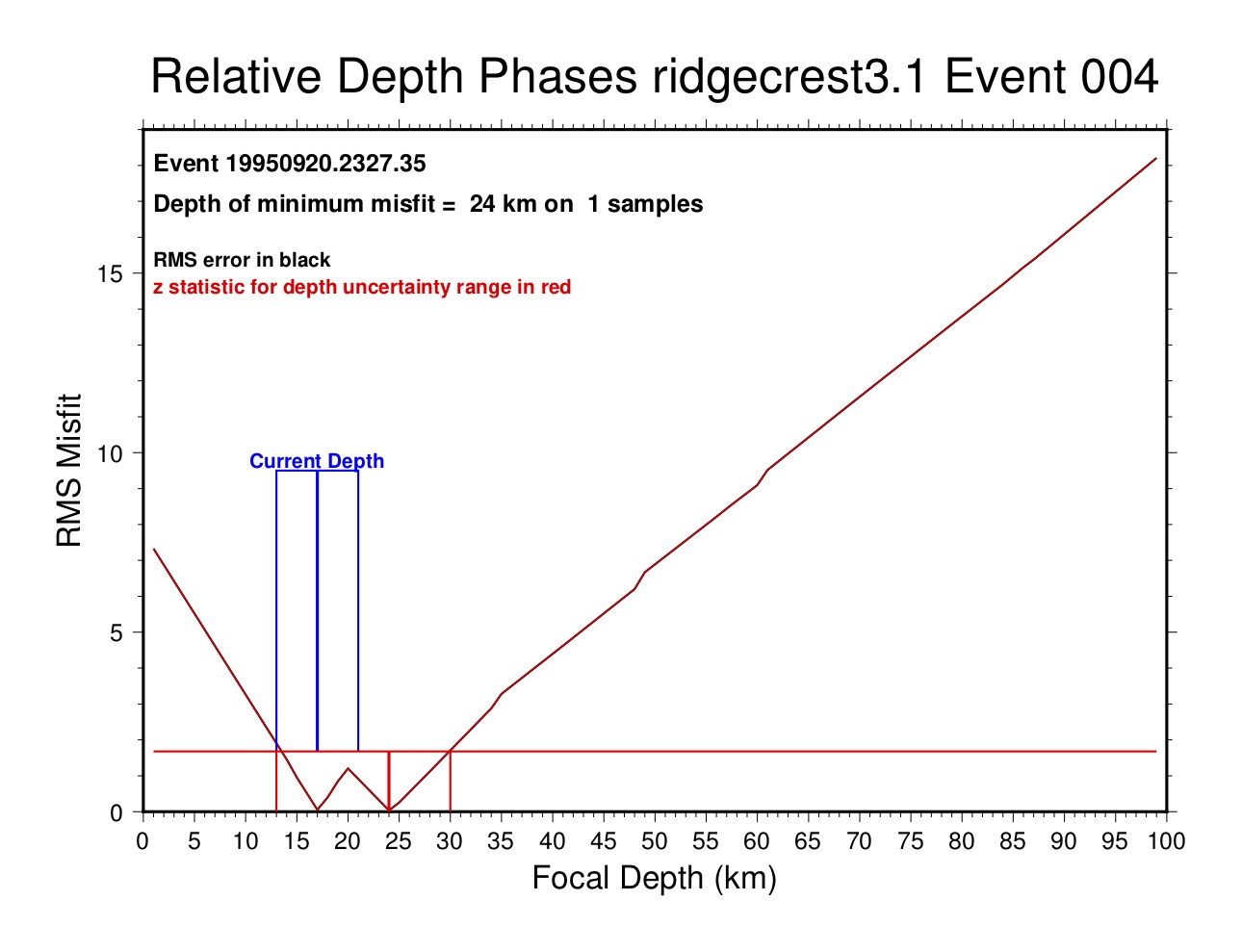
The plot includes two curves, one of the z-statistic (in red) and one (in black) of the total RMS error. For a single datum they are the same. The current depth and uncertainty range is shown in blue. In this case the depth has been set at the shallower minimum (17 km), but not because of the depth phase data; the depth in this run was based on the depl criteria (local distance readings) with an uncertainty of ±4 km.
When there are multiple reports of depth phases there is the possibility (likelihood, actually) of some instances of incompatibility, such as can be seen in the listings above for events 27 and 45. In each case several readings have been flagged after previous runs and now the remaining data are in fair agreement with each other. Experience with a number of events has led to the conclusion that when the squared error term of a reading exceeds 2-3 that reading should probably be flagged. If there are readings with especially large errors (e.g., the sP-P readings for FINES in event 45) they should be flagged first, leaving the “lesser” outliers for consideration after another run.
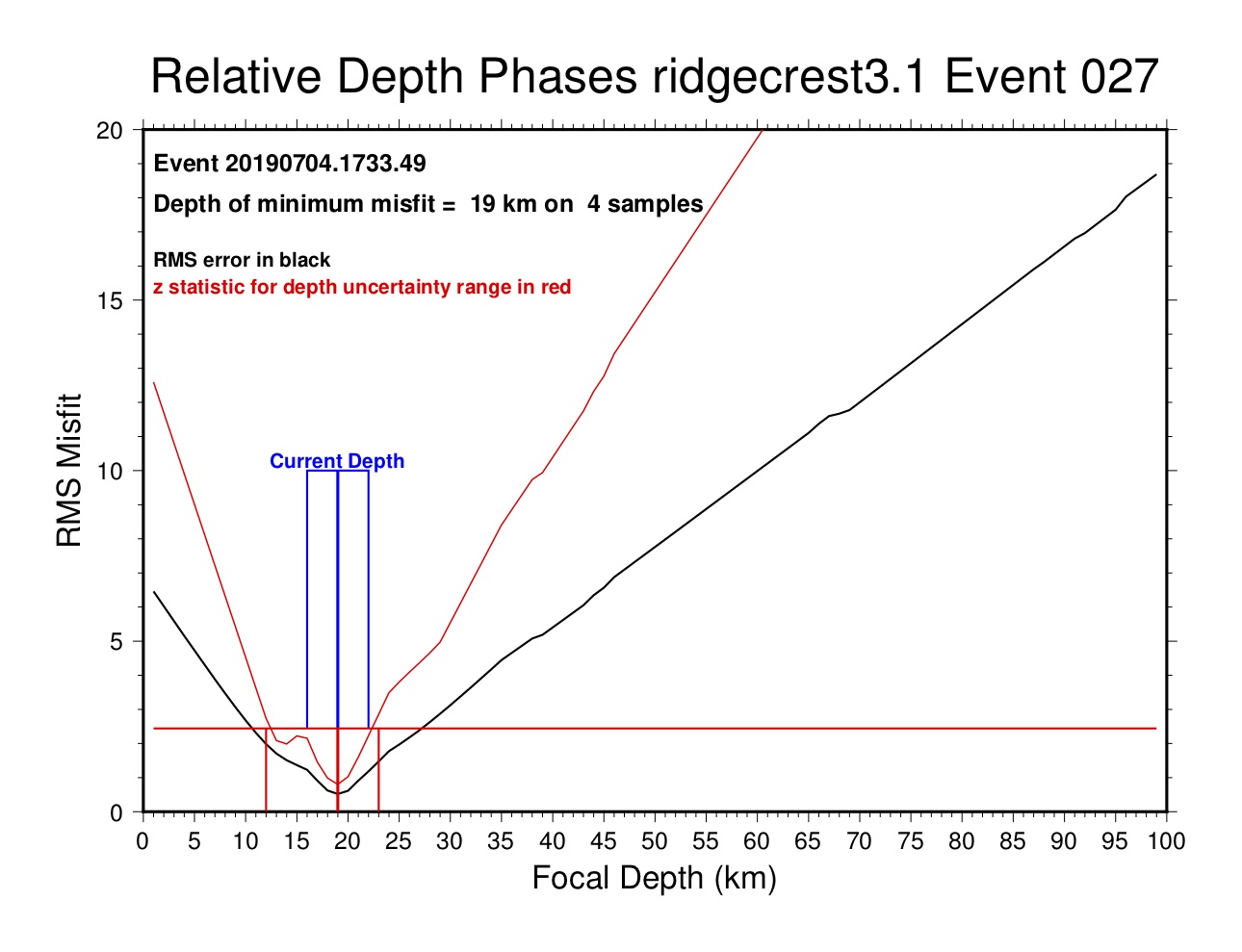
When there are multiple readings the minimum error will usually be non-zero. When outlier readings have been flagged the minimum will usually be less than 2-3. The curves of raw RMS error and the z-statistic will be distinct as well, and the z-statistic always gives a sharper minimum. In this case the preferred depth (19 km) has been set on the basic of near-source readings (depn), but that agrees very well with the depth phase analysis.